A*搜索算法简介及保姆级代码解读

1. A*算法简单介绍

A*算法是一种路径规划算法,和传统的Dijkstra算法有所不同,该算法有选择地进行节点搜索,因此比Dijkstra算法更快、搜索的点更少。
阅读本文,不需要掌握Dijkstra算法的知识,请放心食用。
注意:本文只介绍二维A*算法及相关示例

PS:本文代码编写参考B站up主
小黎的Ally路径规划与轨迹跟踪系列算法学习_第4讲_A*算法,讲解详细,本文代码部分是将其代码进行了些许改动并加以解释,在此对up主的辛苦表达感谢!!

PPS:本文所使用的把地图栅格化的函数来自于博客
Matlab中将一幅图片做成栅格地图,本文进行了些许改动,再次一并感谢博主的辛苦!

1.1 A*算法理论基础

A*算法首先将要搜索的区域划分为若干栅格(grid),并有选择地标识出障碍物(Obstacle)与空白区域。一般地,栅格划分越细密,搜索点数越多,搜索过程越慢,计算量也越大;栅格划分越稀疏,搜索点数越少,相应地搜索精确性就越低
地图栅格

如上图,引入地图信息后画出栅格,该图片采用 100 × 100 100 \times 100 100×100的栅格划分,图中黑色区域为障碍物区域。图中绿点为起始点,红点为终点。

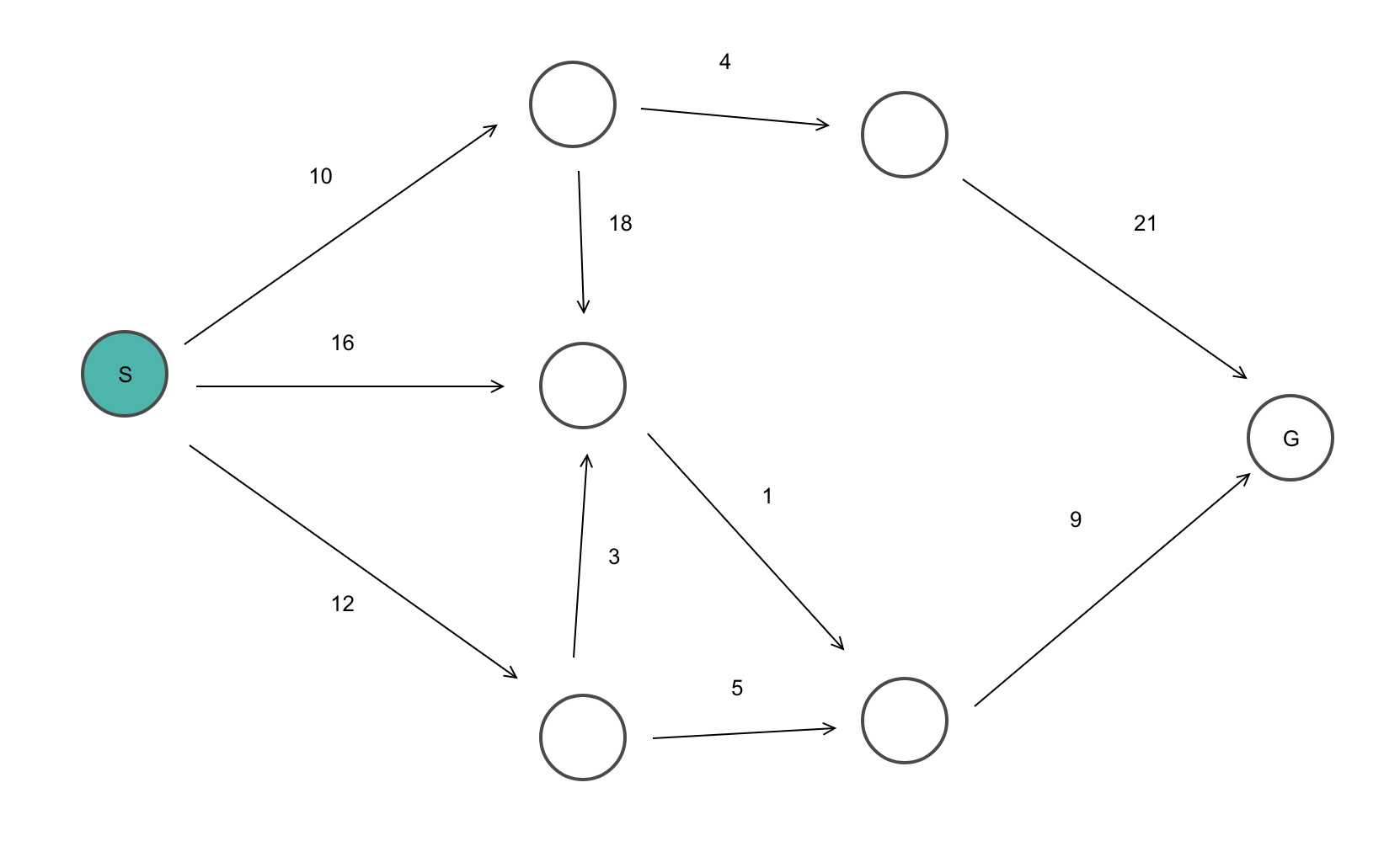
对每个节点,在计算时同时考虑两项代价指标:当前节点与起始点的距离,以及当前节点与目标点的距离
f = g + h f = g + h f=g+h其中 f f f为总代价, g g g为当前节点距离起始点的距离, h h h为当前节点距离目标点的距离。
而在计算距离时,又可以采用两种方式:
欧氏距离
L = ( x 1 − x 2 ) 2 + ( y 1 − y 2 ) 2 L = \sqrt{\left( x_1 - x_2 \right) ^2 + \left( y_1 - y_2 \right) ^2} L=(x1​−x2​)2+(y1​−y2​)2 ​曼哈顿距离
L = ∣ x 1 − x 2 ∣ + ∣ y 1 − y 2 ∣ L = \lvert x_1 - x_2 \rvert + \lvert y_1 - y_2 \rvert L=∣x1​−x2​∣+∣y1​−y2​∣为了计算方便,本文计算 h h h时采用曼哈顿距离,这也是A*算法中的一贯做法。
为了方便计数,在计算每一个节点时,在栅格左上角写 f f f值,左下角写 g g g值,右下角写 h h h值。

1.1.1 节点计算

这里举一个例子。
节点计算例1
如图所示,A点为起始点,M点为终点。对于A点来说,对其周边的8个节点进行寻找,A点本身为父节点,周边8个点为子节点

假设:

  • 格子边长为10,这样水平和竖直位移一格为10,而对角位移一格为14;
  • 从父节点到子节点可以水平、竖直、对角线位移计算 g g g值,而从子节点到目标点只能使用水平、竖直位移计算曼哈顿距离 h h h值。

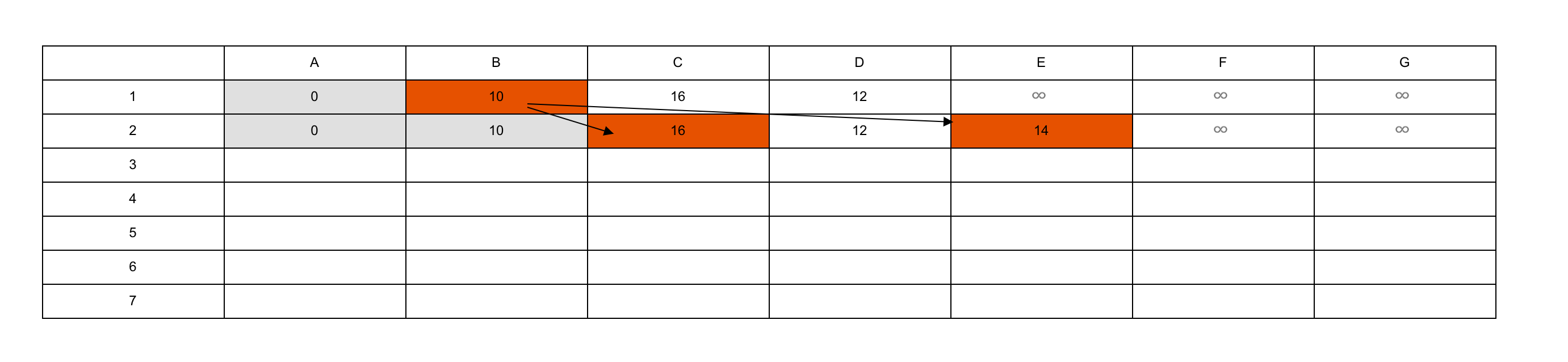
对于点B:从A到B只需右移一格,因此B的 g = 10 g=10 g=10;从B到M需要先右移四格,再上移三格,因此B的 h = 40 + 30 = 70 h = 40+30=70 h=40+30=70。这样B的 f = g + h = 10 + 70 = 80 f=g+h=10+70=80 f=g+h=10+70=80。将三者都记在B格中。
对于点C:从A到C只需向右上方平移一格,因此C的 g = 14 g=14 g=14;从C到M需要先右移四格,再上移两格,因此C的 h = 40 + 20 = 60 h=40+20=60 h=40+20=60,继而C的 f = g + h = 74 f=g+h=74 f=g+h=74。
同理可以计算出D的 g = 14 , h = 80 , f = 94 g=14, h=80,f=94 g=14,h=80,f=94,以及其他几个子节点的值。

将这8个子节点进行对比,可以发现,C点的 f f f值最小,因此选取C点为下一步搜寻的父节点, A C ‾ \overline{AC} AC即为路径迈出的第一步。
节点计算例2
如图所示,现在将C作为新的父节点。

对于J点:
从C到J只需右移一格,因此J的 g = 10 + g C = 10 + 14 = 24 g=10+g_C =10+14=24 g=10+gC​=10+14=24。需要注意的是,J点的 g g g值是从C到J的 g g g加上从A到C的 g g g,即当前子节点的 g g g值是从起点到该点的所有 g g g累和
从J到M需要先右移三格,再上移两格,因此J的 h = 30 + 20 = 50 h = 30+20=50 h=30+20=50。这样J的 f = g + h = 24 + 50 = 74 f=g+h=24+50=74 f=g+h=24+50=74。将三者都记在J格中。

对于I点:
从C到I只需向右上方平移一格,同样地,I点的 g g g值是从C到I的 g g g加上从A到C的 g g g,即当前子节点的 g g g值是从起点到该点的所有 g g g累和,因此I的 g = 14 + g C = 14 + 14 = 28 g=14+g_C =14+14=28 g=14+gC​=14+14=28。
从I到M需要先右移三格,再上移一格,因此I的 h = 30 + 10 = 40 h = 30+10=40 h=30+10=40。这样I的 f = g + h = 28 + 40 = 68 f=g+h=28+40=68 f=g+h=28+40=68。将三者都记在I格中。
同样计算出其他点的值。
可以看出,I点的 f f f值最小,因此选择I点作为路径上的下一个点,此时路径变为 A C I ‾ \overline{ACI} ACI。

如此一步步进行迭代,最后找到最优轨迹。

1.1.2 由计算得出的小结论

  • 每个节点中需要存储至少3个值: g , h , f g,h,f g,h,f。
  • 当子节点迭代到目标点本身时, h = 0 h=0 h=0,即当前节点到目标点的距离为0.
  • 在算法实施时, g g g的计算可以取10或14,即从父节点到子节点可以水平/竖直位移,也可以沿对角线位移;而 h h h的计算只能取10的倍数,即从当前子节点到目标点只能水平/竖直位移。前者可以采用欧氏距离,后者只能采用曼哈顿距离
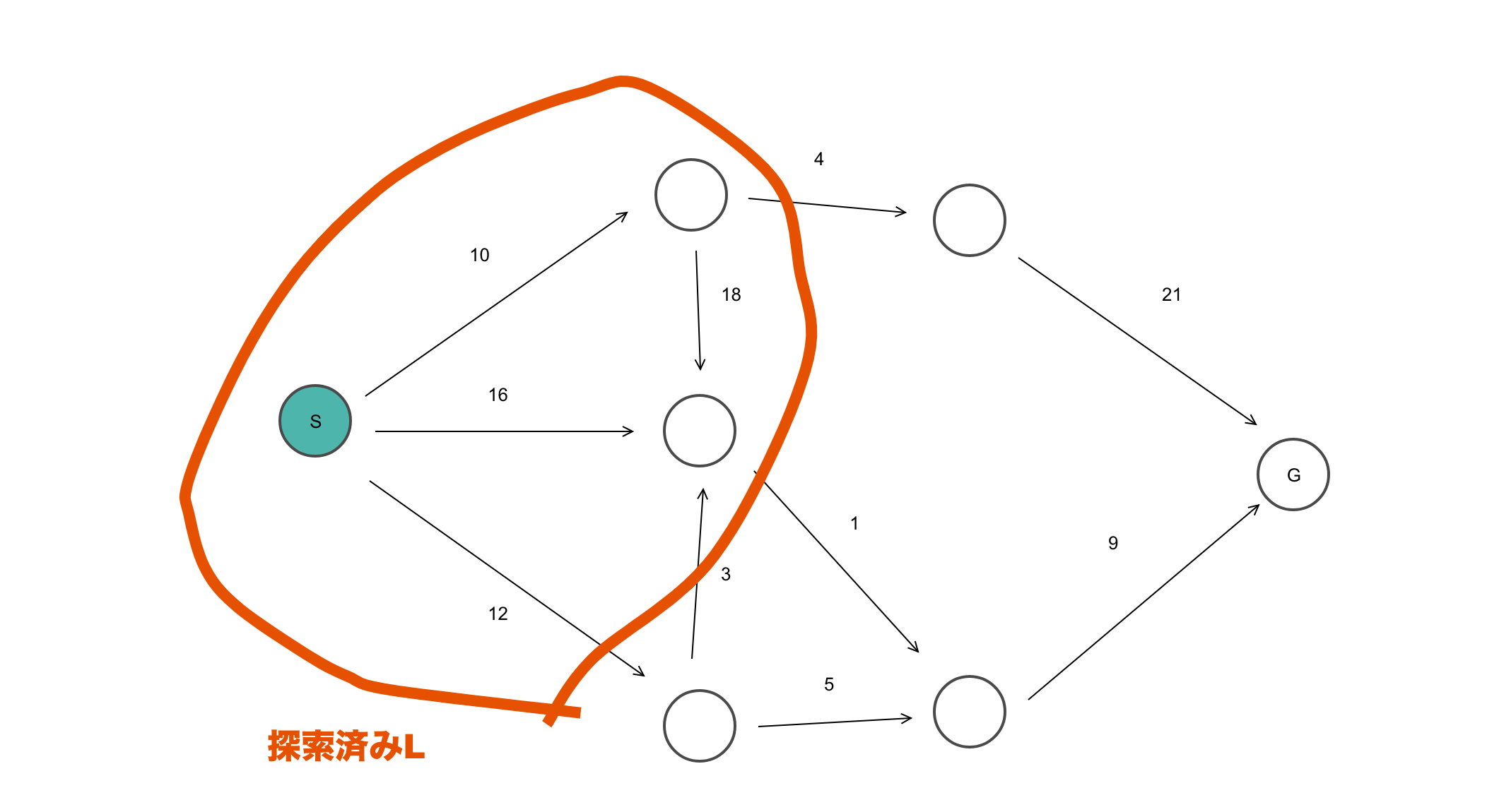
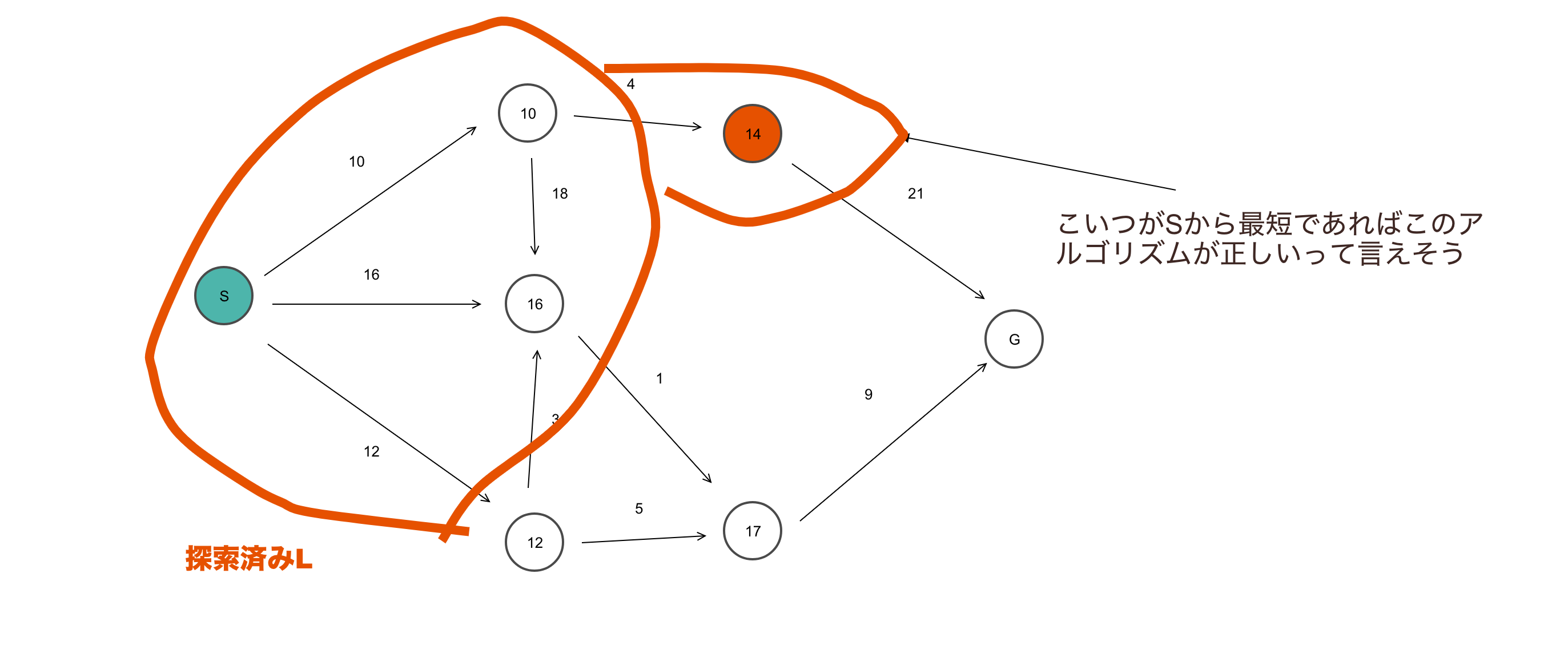
  • 当某个子节点被选中后,就作为下一次搜索的父节点;并且为了避免节点的重复计算和筛选,在下一次搜索时,需要将上一步选中的节点从“可搜索”列表中删除。如上图中,当C为父节点时,选中I作为下一次的父节点;那么当第二步I为父节点时,由于C已经在已选轨迹上了,所以I的子节点实际上并不包括C,只计算7个子节点即可。
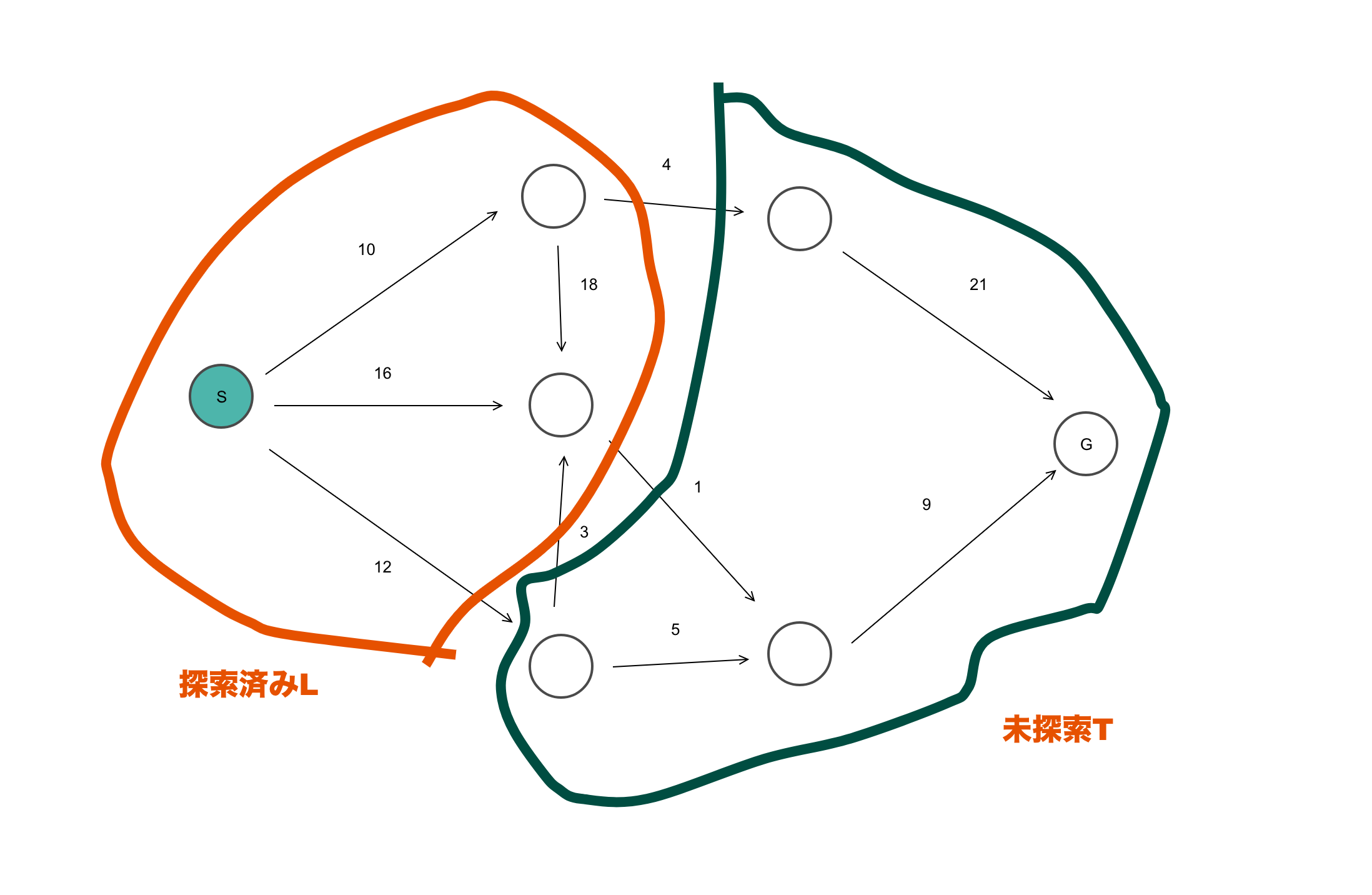
  • 鉴于上一点,可以预想,算法的具体实施过程中,需要有两个数组保存“待计算子节点”和“已被选中的节点”。当“待计算子节点”中某个点符合 f f f最小时,就将其加入“已选中的节点”,并在“待计算子节点”中删除该点,防止后续重复计算
  • 当算法结束时,保存在“已选中的节点”中的所有点,按照顺序即为找出的路径
  • 算法结束时,最后一个点的 f f f值,即为从起点到终点所用的距离
  • 算法的停止条件:1)当“待计算子节点”中没有点时,即已经没有点可供寻找了;2)当当前父节点恰为目标节点时,即 h = 0 h=0 h=0。

1.2 算法逻辑结构

A*算法的逻辑结构如下:
1)初始化。导入地图信息,设置障碍物区域,设置起点start、终点target、栅格数量 m × n m \times n m×n等。
2)数据预处理。建立“待计算子节点”的数组openlist,“已选中的节点”的数组closelist,保存路径的数组closelist_path。除此之外,还需建立一个当前子节点集合children,用来保存当前父节点周围8个子节点的坐标,以及父节点本身parent;还有保存代价值 g , h , f g, h,f g,h,f的数组openlist_costcloselist_cost
3)对子节点们children中的每个节点child
若该子节点不在“待计算子节点”节点openlist中,则追加进去;
若在,则计算出该child的 g g g值,该 g g g值是从起点到父节点parent的距离加上父节点到该子节点的距离。若该 g g g值小于之前openlist_cost中的 g g g最小值,那么就将openlist_cost中的最小 g g g值更新;
4)由于该代价最小点已经加入了轨迹,因此将该点加入clost_listcloselist_path,并从openlist中剔除;
5)更新openlist中的最小代价值,并以其为父节点开始新一轮搜索。

2. 代码解析

2.1 引入地图

代码块:

1
2
3
4
5
6
7
8
9
10
11
12
13
14
15
16
17
18
19
20
21
22
23
24
25
26
27
28
29
30
31
32
33
34
35
36
37
38
39
40
%% 画地图

% 栅格地图的行数、列数定义
m = 150;
n = 150;
% 地图m行n列

start = [10, 20]; % 起始节点
target = [130, 80]; % 终止节点

obs = TrunToGridMap(m, n);


% 画格子
for i = 0 : 5 : m
plot([0, n], [i, i], 'k', 'handlevisibility', 'off');
hold on;
end

for j = 0 : 5 : n
plot([j, j], [0, m], 'k', 'handlevisibility', 'off');
end

axis equal;
xlim([0, n]);
ylim([0, m]);

% 绘制障碍物、起止点颜色块
scatter(start(1), start(2), 700, 'pg', 'filled');
scatter(target(1), target(2), 700, 'pr', 'filled');

for i = 1 : size(obs, 1) - 1
temp = obs(i, :);
fill([temp(1)-1, temp(1), temp(1), temp(1)-1],...
[temp(2)-1, temp(2)-1, temp(2), temp(2)], 'k', 'handlevisibility', 'off');
end

temp = obs(size(obs, 1), :);
fill([temp(1)-1, temp(1), temp(1), temp(1)-1],...
[temp(2)-1, temp(2)-1, temp(2), temp(2)], 'k');

绘制一个 150 × 150 150 \times 150 150×150的地图,起点设置为 ( 10 , 20 ) (10,20) (10,20),终点设置为 ( 130 , 80 ) (130,80) (130,80)。
障碍物的坐标通过函数TrunToGridMap(m, n)获得:

1
2
3
4
5
6
7
8
9
10
11
12
13
14
15
16
17
18
19
20
21
22
23
24
25
26
27
28
function obs = TrunToGridMap(a, b)
I=imread('此处放地图图片的文件名'); %读入图片
I = rgb2gray(I); %将图片转为灰度图
I = imrotate(I, -90);

l=1; %网格边长
B = imresize(I,[a/l b/l]);
J=floor(B/255);

axes('GridLineStyle', '-');
axis equal;

hold on
grid on
axis([0,a,0,b]);
set(gca,'xtick',0:10:a,'ytick',0:10:b);

obs = [];

%障碍物填充为黑色
for i=1:a/l-1
for j=1:b/l-1
if(J(i,j)==0)
obs(end+1, :) = [i, j];
end
end
end
end

该函数读取一个图片文件,将其转化为灰度图像,并将灰度图中黑色色块所在的坐标返回为障碍物坐标。

2.2 预处理

1
2
3
4
5
6
7
8
9
10
11
12
13
14
15
16
17
18
19
20
21
22
23
%% 预处理

% 初始化closelist
closelist = start;
closelist_path = {start, start}; % 路径,从自身到自身
closelist_cost = 0;
children = child_nodes_cal(start, m, n, obs, closelist);

% 初始化openlist
openlist = children;


for i = 1 : size(openlist, 1) % i为第i个节点
openlist_path{i, 1} = openlist(i, :); % openlist_path的第i行第1列为第i个节点child
openlist_path{i, 2} = [start; openlist(i, :)]; % openlist_path的第i行第2列为一个列向量,分别是起始节点和当前child
end

for i = 1 : size(openlist, 1)
g = norm(start - openlist(i, 1:2));
h = abs(target(1) - openlist(i, 1)) + abs(target(2) - openlist(i, 2));
f = g + h;
openlist_cost(i, :) = [g, h, f];
end

这一部分主要做了以下几步:

  • 把起点start设为轨迹的第一个点:closelist = start
  • 路径初始化,即从起点到起点:closelist_path = {start, start}
  • 代价首先置为0:closelist_cost = 0
  • 利用child_nodes_cal函数计算当前父节点(即起点)周围的子节点们;
  • 这些子节点们children即为待计算的子节点,也就是openlist
  • 随后进入一个循环,对每一个子节点i,openlist_path中第i行第1个元素储存第i个节点child,第2个元素为一个列向量,分别是第i个child的起点和它本身;
  • 第二个循环则是计算代价的循环,对每一个子节点i,计算 g g g(这里使用范数norm), h h h(曼哈顿距离)和 f f f;之后,在代价数组openlist_cost中储存这三个代价值,因此openlist_cost第i行的元素为一个行向量

其中用到的子节点计算函数如下:

1
2
3
4
5
6
7
8
9
10
11
12
13
14
15
16
17
18
19
20
21
22
23
24
25
26
27
28
29
30
31
32
33
34
35
36
37
38
39
40
41
42
43
44
45
46
47
48
49
50
51
52
53
54
55
56
57
58
59
60
61
62
63
64
65
66
67
68
69
70
71
72
73
74
75
76
77
78
79
80
81
82
83
84
85
86
87
88
89
function child_nodes = child_nodes_cal(parent_node, m, n, obs, closelist)
child_nodes = [];
field = [1, 1;
n, 1;
n, m;
1, m];

% 左上子节点
child_node = [parent_node(1) - 1, parent_node(2) + 1];
if inpolygon(child_node(1), child_node(2), field(:, 1), field(:, 2))
% [in, on] = inpolygon, 返回 in,以指明 xq 和 yq 所指定的查询点是在 xv 和
% yv 定义的多边形区% 域的边缘内部还是在边缘上,in为内部,on为边缘上
if ~ismember(child_node, obs, 'rows')
child_nodes = [child_nodes; child_node];
end
end


% 上子节点
child_node = [parent_node(1), parent_node(2) + 1];
if inpolygon(child_node(1), child_node(2), field(:, 1), field(:, 2))
if ~ismember(child_node, obs, 'rows')
child_nodes = [child_nodes; child_node];
end
end


% 右上子节点
child_node = [parent_node(1) + 1, parent_node(2) + 1];
if inpolygon(child_node(1), child_node(2), field(:, 1), field(:, 2))
if ~ismember(child_node, obs, 'rows')
child_nodes = [child_nodes; child_node];
end
end

% 左子节点
child_node = [parent_node(1) - 1, parent_node(2)];
if inpolygon(child_node(1), child_node(2), field(:, 1), field(:, 2))
if ~ismember(child_node, obs, 'rows')
child_nodes = [child_nodes; child_node];
end
end

%右子节点
child_node = [parent_node(1) + 1, parent_node(2)];
if inpolygon(child_node(1), child_node(2), field(:, 1), field(:, 2))
if ~ismember(child_node, obs, 'rows')
child_nodes = [child_nodes; child_node];
end
end


%左下子节点
child_node = [parent_node(1) - 1, parent_node(2) - 1];
if inpolygon(child_node(1), child_node(2), field(:, 1), field(:, 2))
if ~ismember(child_node, obs, 'rows')
child_nodes = [child_nodes; child_node];
end
end


% 下子节点
child_node = [parent_node(1), parent_node(2) - 1];
if inpolygon(child_node(1), child_node(2), field(:, 1), field(:, 2))
if ~ismember(child_node, obs, 'rows')
child_nodes = [child_nodes; child_node];
end
end


% 右下子节点
child_node = [parent_node(1) + 1, parent_node(2) - 1];
if inpolygon(child_node(1), child_node(2), field(:, 1), field(:, 2))
if ~ismember(child_node, obs, 'rows')
child_nodes = [child_nodes; child_node];
end
end


%% 排除已经存在于closelist的节点
delete_idx = [];
for i = 1 : size(child_nodes, 1)
if ismember(child_nodes(i, :), closelist, 'rows')
delete_idx(end+1, :) = i;
end
end

child_nodes(delete_idx, :) = [];
end

2.3 定义父节点parent

1
2
3
4
%% 定义父节点
% 从openlist开始搜索移动代价最小的节点
[~, min_idx] = min(openlist_cost(:, 3)); % 看f值最小,min_idx为f最小的那一行
parent = openlist(min_idx, :);% 以min_idx该行的子节点child_node为新的父节点

这一步搜索openlist_cost代价数组中 f f f最小的元素,记下其索引min_idx
随后该索引对应的openlist中的元素即为“ f f f值最小的待计算子节点”,作为下一步计算的父节点parent

2.4 主循环

1
2
3
4
5
6
7
8
9
10
11
12
13
14
15
16
17
18
19
20
21
22
23
24
25
26
27
28
29
30
31
32
33
34
35
36
37
38
39
40
41
42
43
44
45
46
47
48
49
50
51
52
53
54
55
56
57
58
59
%% 进入循环
flag = 1;
while flag
% 找出父节点的忽略closelist的子节点
children = child_nodes_cal(parent ,m, n, obs, closelist);

% 判断这些子节点是否在openlist中,若在,则更新;没在,则追加到openlist中
for i = 1 : size(children, 1)
child = children(i, :);
[in_flag, openlist_idx] = ismember(child, openlist, 'rows');
% in_flag表示该child_node是否在openlist中
% openlist_idx表示该child_node在openlist中的行数

g = openlist_cost(min_idx, 1) + norm(parent - child);
% 原来的g加上新的g
h = abs(child(1) - target(1)) + abs(child(2) - target(2));
f = g + h;

if in_flag % 若在,则比较更新g, f
if g < openlist_cost(openlist_idx, 1)
% openlist_cost(openlist_idx,1)指的是openlist_cost中idx这一行(即child_node所在的一行)的第一个坐标,即g
openlist_cost(openlist_idx, 1) = g;
openlist_cost(openlist_idx, 3) = f;
openlist_path{openlist_idx, 2} = [openlist_path{min_idx, 2}; child];
% openlist_path的第i行第2列为一个列向量,分别是起始节点和当前child,此处定义新的起始节点为openlist_path(min_idx,2), 而openlist_path(min_idx,2)指第min_idx行所对应的 child在openlist_path中对应的路径,相当于把新的child附加到了路径上,延长了路径
end
else
openlist(end+1, :) = child;
openlist_cost(end+1, :) = [g, h, f];
openlist_path{end+1, 1} = child;
openlist_path{end, 2} = [openlist_path{min_idx, 2}; child];
end
end


% 从openlist移除代价最小的节点到closelist
closelist(end+1, :) = openlist(min_idx, :);
closelist_cost(end+1, :) = openlist_cost(min_idx, 3);
closelist_path(end+1, :) = openlist_path(min_idx, :);

% 同样地,openlist中少了该节点
openlist(min_idx, :) = [];
openlist_cost(min_idx, :) = [];
openlist_path(min_idx, :) = [];


% 重新搜索:从openlist搜索移动代价最小的节点,作为新的父节点
[~, min_idx] = min(openlist_cost(:, 3));
parent = openlist(min_idx, :);

% 判断是否搜索到终点
if parent == target
closelist(end+1, :) = openlist(min_idx, :);
closelist_cost(end+1, 1) = openlist_cost(min_idx, 1);
closelist_path(end+1, :) = openlist_path(min_idx, :);
flag = 0;
end

end

2.4.1

对这一部分循环来说,首先利用child_nodes_cal函数得出当前父节点parent周围的子节点们children
对每一个子节点child,判断其是否在“待计算子节点”openlist列表中——in_flag=1表示在列表中,同时openlist_idx为该子节点在openlist中的索引号。
判断完成后,首先计算该子节点的 g , h , f g,h,f g,h,f值,注意: g g g值为父节点parent的 g g g加上该child子节点的 g g g值。

2.4.2

计算 g , h , f g,h,f g,h,f之后,再来看子节点在openlist中的情况。由于循环中查看了parent周围所有子节点的情况,所以一定会存在某个子节点的 g g g比其他子节点的 g g g都小。如果找到了这样的子节点,那么就更新该子节点在openlist_cost中对应位置的 g , h , f g,h,f g,h,f值。

同时,还要将该子节点加入到路径openlist_path中,即这一句代码

1
openlist_path{openlist_idx, 2} = [openlist_path{min_idx, 2}; child];

这行代码的含义是:
openlist_idx表示当前子节点childopenlist中的索引,min_idx表示之前所有子节点中代价最小的子节点的索引。之前在预处理一节中提到,openlist_path的第i行第2列为一个列向量,分别是父节点和当前child,相当于第2列储存了路径。

min_idx表示“代价最小的节点”,也就是父节点parent。因此这里openlist_path{min_idx, 2}表示父节点的路径。而[openlist_path{min_idx, 2}; child]则是把新的child附加到这一个列向量上,相当于把新的child附加到路径尾端,把向量长度延长了一个child,延长了路径。

这样,[openlist_path{min_idx, 2}; child]构成了一个“父节点路径-当前child”的新路径

把这个新路径赋值给openlist_idx索引所对应的openlist_path上,即为该openlist_idx索引对应的子节点的路径。

2.4.3

另一方面,如果该child不在openlist中,那么就把该child添加到“待计算子节点”列表中,其 g , h , f g,h,f g,h,f值添加到openlist_cost代价列表中,其路径[openlist_path{min_idx, 2}; child]添加到路径openlist_path中。

2.4.4

由于移动代价最小的节点已经是路径上的一点了,所以为了避免重复计算,应当把她从“待计算子节点”列表中删除,加入“已计算节点”中,即

1
2
3
4
5
6
7
closelist(end+1, :) = openlist(min_idx, :);
closelist_cost(end+1, :) = openlist_cost(min_idx, 3);
closelist_path(end+1, :) = openlist_path(min_idx, :);
% openlist中少了该节点
openlist(min_idx, :) = [];
openlist_cost(min_idx, :) = [];
openlist_path(min_idx, :) = [];

仔细观察不难发现,min_idx对应的正是这一步的parent节点,直到这里,我们才把它加入到“已计算节点”列表中,在之前它一直呆在openlist中。

2.4.5

父节点加入到了“已计算节点”中了,那么下一步就没有父节点了,所以需要找出新的父节点:

1
2
 [~, min_idx] = min(openlist_cost(:, 3));
parent = openlist(min_idx, :);

同时还需要判断一下,是否已经进行到了程序结束:

1
2
3
4
5
6
7
% 判断是否搜索到终点
if parent == target
closelist(end+1, :) = openlist(min_idx, :);
closelist_cost(end+1, 1) = openlist_cost(min_idx, 1);
closelist_path(end+1, :) = openlist_path(min_idx, :);
flag = 0;
end

需要注意,即使当当前父节点已经是目标点了,也不要忘了把这个父节点加入到“已计算节点”中,相当于把目标点添加入路径中,形成路径上最后一个点。

2.5 画图

这一步就是将结果绘制出来了:

1
2
3
4
5
6
7
8
9
path_opt = closelist_path{end, 2};
% closelist_path中第二列存放路径,所以path_opt存放的是路径的(x,y)值
path_opt(:, 1) = path_opt(:, 1) - 0.5;
path_opt(:, 2) = path_opt(:, 2) - 0.5;
plot(path_opt(:, 1), path_opt(:, 2), 'm', 'linewidth', 1.5);

title(['Total length of path: ' num2str(closelist_cost(end, 1))]);
legend('Start node', 'Target node', 'Obstacle', 'Path', 'location', 'northwest');
set(gca, 'fontsize', 35, 'fontname', 'times new roman');

3. 结果

这里导入稻妻地图作为路径规划的示例,该地图多为岛屿,路径复杂,障碍物分散且数量多,十分适合作为示例使用。
稻妻地图
将其灰度化得到
灰度稻妻
把地图划分为 m × n = 150 × 150 m \times n = 150 \times 150 m×n=150×150的栅格,并设置起点为 ( 10 , 20 ) (10,20) (10,20),终点为 ( 130 , 80 ) (130,80) (130,80):
稻妻地图栅格
图中绿色为起点,红色为终点。

路径规划结果:
稻妻路径规划
可以看出,A* 算法可以找到期望路径。

文件所有代码在笔者的资源二维A*算法路径规划matlab代码中可以下载得到。

留言與分享

Dijkstra简单介绍

分類 算法

不是有个叫迪杰斯特拉(Dijkstra)的算法吗?名字难记不说,加权图的最短路径问题在实际开发中也很少需要自己实现,所以总是很快就忘了。。。

迪杰斯特拉算法是什么

迪杰斯特拉算法是一种用于求解图的最短路径的算法。很多人可能只是听过这个名字。虽然它的原理简单易懂,但初次接触可能有些难以理解,不过只要逐步分析就会发现它其实是一个相当直观的算法。
对于没有权重的迷宫搜索等问题,可以用广度优先搜索(BFS)解决,但如果每条边都有权重,就需要计算所有可能的路径。假设每个顶点只经过一次,且有E条边,那么时间复杂度会是O(E!),计算量会爆炸式增长。
这样计算起来就很不现实。

而迪杰斯特拉算法正是高效解决这类问题的算法。

需要注意的是,各边的成本必须是非负值(大于等于0)。如果包含负数,则需要使用贝尔曼-福特(Bellman-Ford)等算法。

步骤

迪杰斯特拉算法的步骤非常简单:

  1. 将起点的最短距离设为0
  2. 从未访问的点中选择已知最短距离且距离最小的顶点移动
  3. 设置该顶点连接的其他顶点的最短距离。如果可以更新更短的距离,则更新。
  4. 重复以上步骤,直到所有顶点的最短距离都确定

光这么说可能有点抽象,下面我们通过一个具体例子来说明。

示例

虽然方法很原始,但这是最能表达清楚的方式…
我们来看下面这张图的最短路径:
image.png

绿色表示最短路径已确定并已访问的顶点,红色是起点顶点。每个顶点上的数字表示当前的最短路径:
dijkstra algo.gif

可以看到,算法从起点开始,每次移动到当前最短路径的顶点,并计算相邻顶点的最短路径。

实现

接下来我们来实现这个算法。
按照上述步骤直接实现:

1
2
3
4
5
6
7
8
9
10
11
12
13
14
15
16
17
18
19
20
21
22
23
24
25
26
27
28
29
30
31
32
33
34
35
36
37
38
function main(nodes) {
const start = nodes[0]
// 记录已访问的顶点
const visited = new Set()
const routesFromStart = new Map()
// 记录从起点出发的距离

routesFromStart.set(start, {distance: 0})
for(const n of nodes) {
if(n != start) {
// 除起点外所有顶点初始化为无穷大
routesFromStart.set(n, {distance: Number.MAX_VALUE})
}
}
let current = start
let routes = new Map()
while(current != null) {
visited.add(current)
for(const edge of current.edges) {
// 计算相邻顶点的最短距离,如果更小则更新
if(edge.cost + routesFromStart.get(current).distance < routesFromStart.get(edge.to).distance) {
routesFromStart.set(edge.to, {distance: edge.cost + routesFromStart.get(current).distance})
routes.set(current, edge.to)
}
}
let cheapestNodeDistance = Number.MAX_VALUE
current = null
// 从已计算最短距离的未访问顶点中选择最小的顶点

for(const city of routesFromStart.keys()) {
if(!visited.has(city) && cheapestNodeDistance > routesFromStart.get(city).distance){
cheapestNodeDistance = routesFromStart.get(city).distance
current = city
}
}
}
return routesFromStart.get(nodes[nodes.length - 1]).distance
}

假设顶点数为V,这段代码在最坏情况下需要遍历所有边,并在内部循环中选择最小顶点,因此时间复杂度是O(V² + E)。空间复杂度需要记录每个顶点,所以是O(V)。

关于使用优先队列的实现

细心的读者可能已经发现,这段代码中选取最小顶点的逻辑可以优化,这就是优先队列(Priority Queue)。
优先队列的插入和取出操作需要O(logN)的时间复杂度,但比线性搜索最小顶点更快。

JavaScript没有内置优先队列,以下是Python实现:

1
2
3
4
5
6
7
8
9
10
11
12
13
14
15
16
17
18
19
20
21
22
23
24
25
26
27
28
def dijkstra(nodes):
start_node = nodes[0]
routes_from_start = {n: math.inf for n in nodes}

# 起点距离设为0
routes_from_start[start_node] = 0

minHeap = []

# 添加起点
heappush(minHeap, (0, start_node))

# 直到堆为空
while minHeap:
(cost, current_node) = heappop(minHeap)

# 检查priority key是否重复
if cost > routes_from_start[current_node]:
continue

for node in current_node.routes:
price_info = current_node.routes[node]
if routes_from_start[node] > price_info + routes_from_start[current_node]:
routes_from_start[node] = price_info + routes_from_start[current_node]
# 记录更新最短距离的节点
heappush(minHeap, (price_info + routes_from_start[current_node], node))

return routes_from_start[nodes[-1]]

优先队列的说明我们以后再讨论。
优化后的算法时间复杂度为O(V + ElogE),比最初的实现更高效。

记录路径

现在我们已经能求出最短成本,但这是"最短路径"问题,我们自然还想知道具体路径。
改进上面的代码:

1
2
3
4
5
6
7
8
9
10
11
12
13
14
15
16
17
18
19
20
21
22
23
24
25
26
27
28
29
30
31
32
33
34
35
36
37
38
39
40
def dijkstra(nodes):
start_node = nodes[0]
routes_from_start = {n: math.inf for n in nodes}

# 起点距离设为0
routes_from_start[start_node] = 0

minHeap = []

# 添加起点
heappush(minHeap, (0, start_node))
path = collections.defaultdict(Node)

# 直到堆为空
while minHeap:
(cost, current_node) = heappop(minHeap)

# 检查priority key是否重复
if cost > routes_from_start[current_node]:
continue

for node in current_node.routes:
price_info = current_node.routes[node]
if routes_from_start[node] > price_info + routes_from_start[current_node]:
routes_from_start[node] = price_info + routes_from_start[current_node]
# 记录更新最短距离的节点
path[node.id] = current_node.id
heappush(minHeap, (price_info + routes_from_start[current_node], node))

current_node = nodes[-1].id
path_array = []

# 从终点回溯记录的最短路径节点
while current_node:
path_array.append(current_node)
if current_node not in path:
break
current_node = path[current_node]

return routes_from_start[nodes[-1]], path_array[::-1]

迪杰斯特拉算法会记录更新最短距离的节点,最后回溯即可。时间复杂度会增加最短路径节点数的计算量。

为什么这样能求出最短路径

看到这里,很多人可能会想:算法本身很简单,实现也不难,但为什么能保证求出最短距离呢?我们简单验证一下:

image.png

假设集合L中的顶点到起点S的最短距离已确定,那么从L连接到的最小顶点也应该是S的最短距离。

image.png

image.png

在集合T中选取最小顶点i,则d[i] = min(T)。对于任意顶点k,最短距离d[k] ≥ d[i]是确定的,因为d[i]是最小值且各边权重非负。
通过归纳法可以证明这一点。

其实这就是一个递推公式:

d[i] = min(k ⊂ T) + i到L中相邻顶点的最短距离

说到递推公式就想到动态规划(DP)。关于DP可以参考这篇文章:
https://qiita.com/drken/items/a5e6fe22863b7992efdb

用DP来看值的更新过程:
image.png

纵轴表示迭代次数,横轴表示顶点。原来迪杰斯特拉算法是DP的一种啊。

总结

通过以上分析,迪杰斯特拉算法一旦理解后其实相当简单。以后在算法问题中遇到类似问题时,希望能快速联想到这个算法。
*顺便说一句,我也想写一篇关于DP的文章

讲解视频可以在这里观看:
https://youtu.be/jz8b0q5R1Ss

参考

http://www.lab2.kuis.kyoto-u.ac.jp/~shuichi/algintro/alg-6s.pdf
https://www.youtube.com/watch?v=X1AsMlJdiok

留言與分享

  • 第 1 頁 共 1 頁
作者的圖片

Kein Chan

這是獨立全棧工程師Kein Chan的技術博客
分享一些技術教程,命令備忘(cheat-sheet)等


全棧工程師
資深技術顧問
數據科學家
Hit廣島觀光大使


Tokyo/Macau